vba searching through rows and their associated co

Question

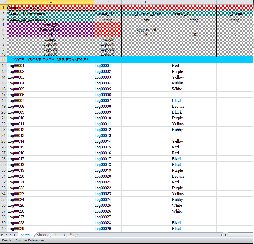
The code below would search through a row and its associated columns. For Row 7, if it is a "N" or "TR" and if all entries are blank below line 12,the code would hide the entire column.

However, I still need help with some further help!

1. If there is a "N" or "TR" in row 7. If there is something writen in any cell, (rather than leaving it alone), can I highlight its associated cell in row 7 in yellow?

2. If ther eis a "Y" in row 7, If there is any empty cells, can I highlight its associated cell in row 7 in yellow?

Thank you so much! special thanks to KazJaw for my previous post about simular issue

Sub checkandhide()

Dim r As Range

Dim Cell As Range

Set r = Range("A7", Cells(7, Columns.Count).End(xlToLeft))

For Each Cell In r

    If Cell.Value = "N" Or Cell.Value = "TR" Then
        If Cells(Rows.Count, Cell.Column).End(xlUp).Row < 13 Then
            Cell.EntireColumn.Hidden = True
        End If
    End If
Next

End Sub

attached example of spreadsheet

Answer 1

Here you have an improved version of your code (although I might need further clarifications... read below).

Sub checkandhide()

    Dim r as Range, Cell As Range, curRange As Range

    Set r = Range("A7", Cells(7, Columns.Count).End(xlToLeft))

    For Each Cell In r

        Set curRange = Range(Cells(13, Cell.Column), Cells(Rows.Count, Cell.Column)) 'Range from row 13 until last row in the given column
        If Cell.Value = "N" Or Cell.Value = "TR" Then
            If Application.CountBlank(curRange) = curRange.Cells.Count Then
                Cell.EntireColumn.Hidden = True
            Else
                Cell.Interior.ColorIndex = 6 'http://dmcritchie.mvps.org/excel/colors.htm
            End If
        ElseIf Cell.Value = "Y" Then
            If Application.CountBlank(curRange) > 0 Then
                 Cell.Interior.ColorIndex = 6 'http://dmcritchie.mvps.org/excel/colors.htm
            End If
        End If
    Next

End Sub

I am not sure if I have understood your instructions properly and thus I will describe here what this code does exactly; please, comment any issue which is not exactly as you want and such that I can update the code accordingly:

It looks for all the cells in range r.

• If the given cell (which might be in row 7 or in any other row below it) meets one of the conditions, the corresponding actions would be performed.
• Part of the conditions depends on curRange, which is defined as all the rows between row number 13 until the end of the spreadsheet.
• Specific conditions:
  a) If the value of the current cell is N or TR. If all the cells in curRange are blank, the current column is hidden. If there is, at least, a non-blank cell, the background color of the given cell would be set to yellow.
  b) If the value of the current cell is Y and there is, at least, one cell in curRange which is not blank, the background color of the background cell would be set to yellow.